Transforming Inventory Levels Into Clean Daily Stock Outflows

Using ASOF joins and linear interpolation

I have previously touched briefly on the process of converting scraped inventory levels into sales estimates, and today I would like to discuss one aspect of that process in more detail.

Imagine we are continuously collecting SKU inventory levels through a scheduled process. Generally, it is better to collect data more frequently, but more frequent data collection has highler collection costs. In some situations the frequency might change over time — we might start collecting data daily and if we find some value, we can increase frequency to get more accurate data. Moreover, when it comes to web scraping, it is not uncommon to have some missing data. Even with the best setup and expertise, many factors are beyond our control, and it always takes time to restore normal operations when something breaks. As far as I know, no one can offer real Service Level Agreements (SLAs) for collecting data from third-party websites. This means we often have to handle some missing data at the data analysis stage, which makes the process of transitioning from collecting inventory levels to measuring daily stock outflows somewhat complex.

This week, I want to discuss how I standardize stock outflows to a specific time frequency (usually daily and sometimes hourly). To achieve this, I use a data transformation process involving ASOF joins and linear interpolation. Let’s break down this transformation process into simple steps.

First, let's examine our source data. For the purposes of this article, I will omit stock replenishments and any other sudden changes in inventory levels — I have already explained how I address these in some of my previous posts:

• Using Web-Extracted Data in Investment Research

• Case Study: Figs Inc (NYSE: FIGS)

I will assume that the input data looks like this:

SELECT
  *
FROM
  raw_inventory_levels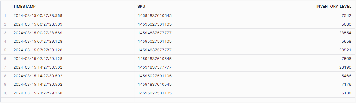

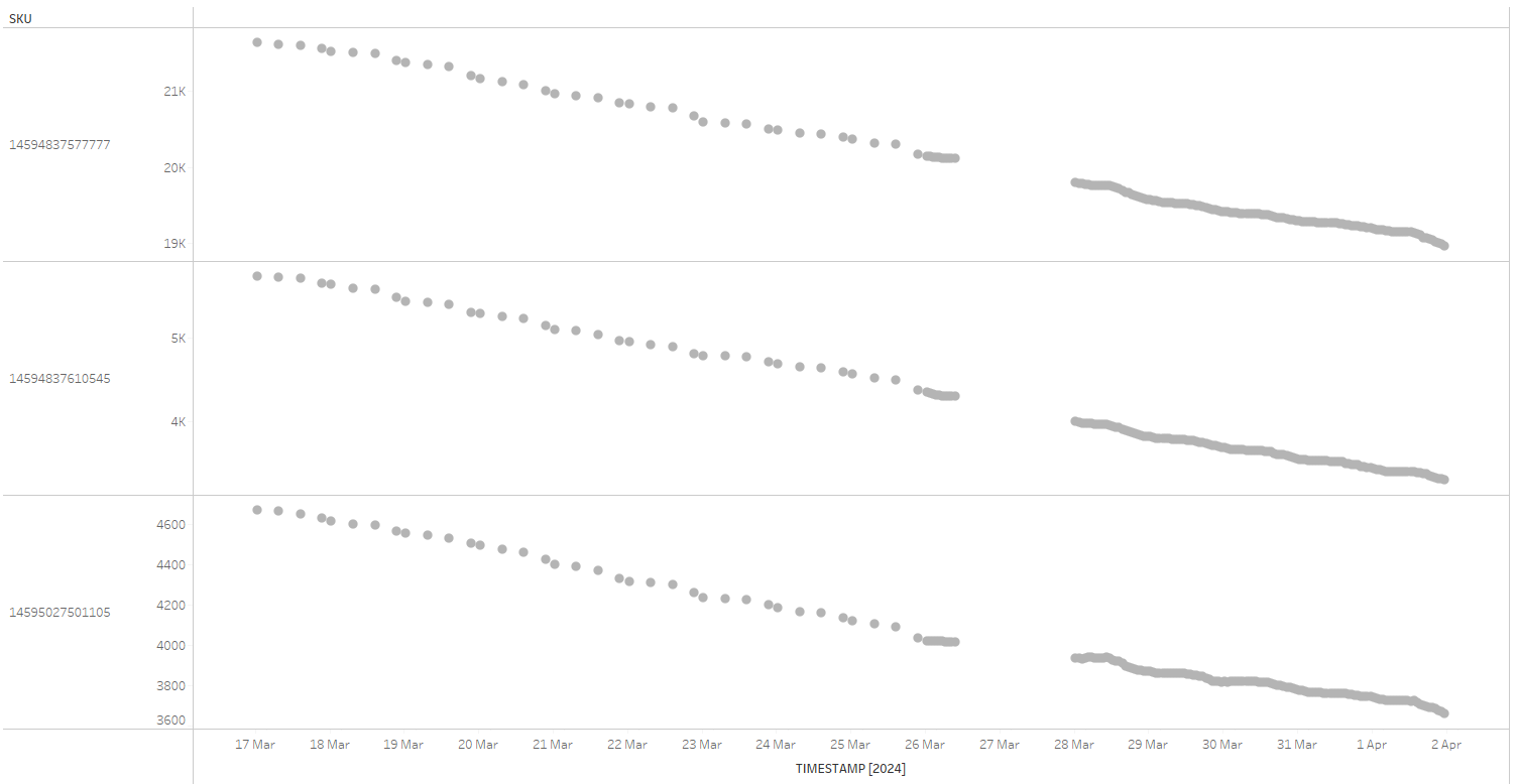
We have measurements of inventory levels, collected for various SKUs at different time intervals. A couple of issues are immediately apparent: the frequency of data collection has increased partway through this time window. It transitioned from approximately three data points per day to hourly data points around May 26. Additionally, there's a complete absence of data on March 27th, likely due to a failed scraping job.

Let’s now transition this raw data into estimated stock outflows.

The first step involves building a 'scaffolding' calendar. This is essentially a series of daily timestamps for each SKU, covering the entire period of interest, set to a predetermined frequency—daily, in this example.

This is achieved with the following Common Table Expression (CTE), which returns a temporary result set that we can reuse in subsequent sections of the SQL query:

WITH calendar AS (
  SELECT 
    DATEADD(day, SEQ4(), start_date) AS date
  FROM 
    TABLE(GENERATOR(ROWCOUNT => 10000)), -- Assume a large enough value
    (SELECT 
        DATE_TRUNC('day', MIN(timestamp)) AS start_date,
        DATE_TRUNC('day', MAX(timestamp)) AS end_date
     FROM 
        raw_inventory_levels) AS date_range
  WHERE 
    DATEADD(day, SEQ4(), start_date) BETWEEN start_date AND end_date
),

calendar_skus AS (
  SELECT
    date,
    sku
  FROM
    calendar
  CROSS JOIN 
    (SELECT DISTINCT sku FROM raw_inventory_levels)
)

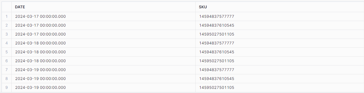
This CTE generates midnight timestamps for each day within our specified time range and for each SKU present in our source data. Importantly, it also includes the days for which data is missing from the source, such as March 27th:

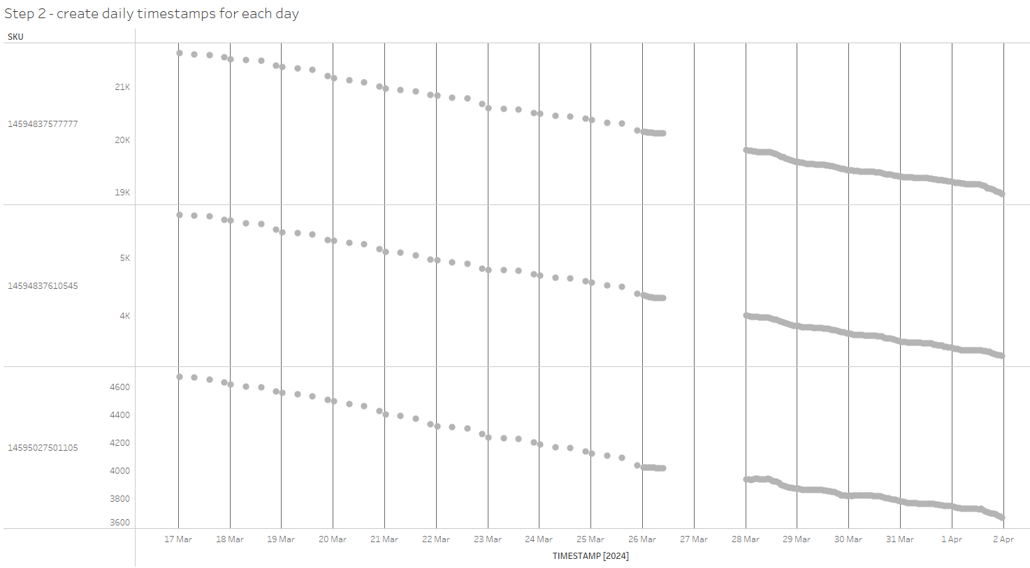
The timestamps are represented as vertical gridlines in the chart, combined with the source data. Initially, these timestamps do not carry any values; they serve merely as a 'helper' structure for the subsequent steps in our analysis.

The next step involves identifying two observations of inventory levels from the source dataset that are closest to each midnight timestamp—one before and one after midnight.

This is where ASOF joins come into play. Without this type of JOIN, we would have to perform a costly operation involving joining all observations for any specific SKU with all timestamps, followed by filtering based on time proximity—a complex and computationally expensive task, especially considering the potential scale involving millions of SKUs, hundreds of days, and thousands of observations.

Instead, we utilize an ASOF join, linking our calendar scaffold with the original inventory levels and including SKU in the join condition. This approach significantly optimizes our data processing by directly aligning each timestamp with the nearest inventory records.

preceding AS (
  SELECT raw_inventory_levels.*,
    calendar_skus.date
  FROM calendar_skus
  ASOF JOIN raw_inventory_levels
  MATCH_CONDITION(calendar_skus.date >= raw_inventory_levels.timestamp)
    ON calendar_skus.sku=raw_inventory_levels.sku
),

succeeding AS (
  SELECT raw_inventory_levels.*,
    calendar_skus.date
  FROM calendar_skus
  ASOF JOIN raw_inventory_levels
  MATCH_CONDITION(calendar_skus.date <= raw_inventory_levels.timestamp)
    ON calendar_skus.sku=raw_inventory_levels.sku
)

This step gives us the two values and corresponding timestamps that are nearest to each midnight timestamp. Below is the result of this step, combined with the previous steps. The coloured marks represent observations closest to the midnight of each day.

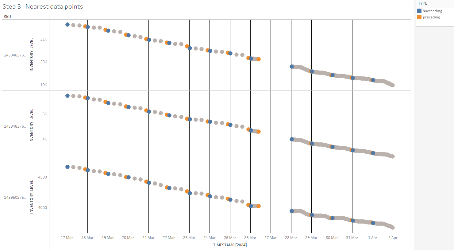
Once we have identified the nearest preceding and succeeding values for each SKU and for each midnight timestamp, we can proceed to estimate the values at midnight using linear interpolation.

Consider the following definitions for the interpolation process:

• t₀ and x₀ represent the time and value before the point of interpolation.

• t₁ and x₁​ represent the time and value after the point of interpolation.

• t is the time at which we want to interpolate the value x.

\(x = x_0 + \frac{(x_1 - x_0)}{(t_1 - t_0)} (t - t_0) \)

Expressing this formula in SQL, we get the following:

interpolation AS (
    SELECT
      preceding.sku,
      preceding.date AS timestamp,
      preceding.inventory_level 
        + (succeeding.inventory_level - preceding.inventory_level)::FLOAT 
        * (timestampdiff('s', preceding.date, preceding.timestamp)::FLOAT 
           / timestampdiff('s', succeeding.timestamp, preceding.timestamp)::float) AS inventory_level
    FROM preceding
    INNER JOIN succeeding
    WHERE
      preceding.sku = succeeding.sku
      AND preceding.date = succeeding.date
)

Optionally, to safeguard against division by zero—a potential issue if our source data contains timestamps exactly at midnight—we can add a very small value to the denominator.

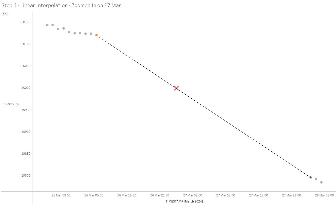
Let’s zoom in on a specific instance: 27 May at 00:00, for one particular SKU, to see what exactly occurs during this step. With linear interpolation, we essentially connect the nearest preceding and succeeding observations with a straight line. We then determine the point where this line intersects with the timestamp of interest (midnight in our case). This process helps us estimate the precise value at this specific moment.

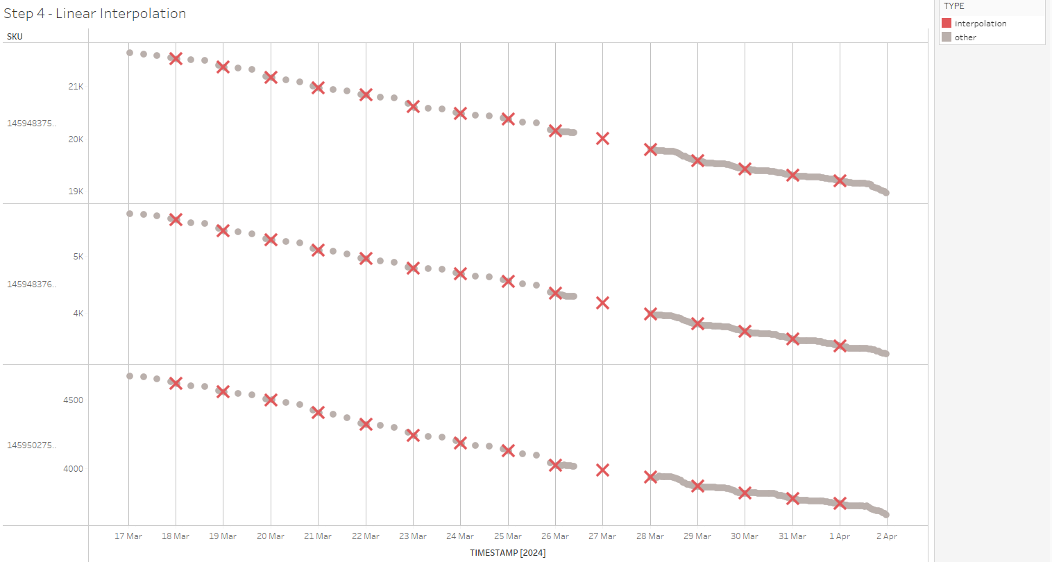
This is the overall result of this step; we now have interpolated daily values for each SKU and for each day:

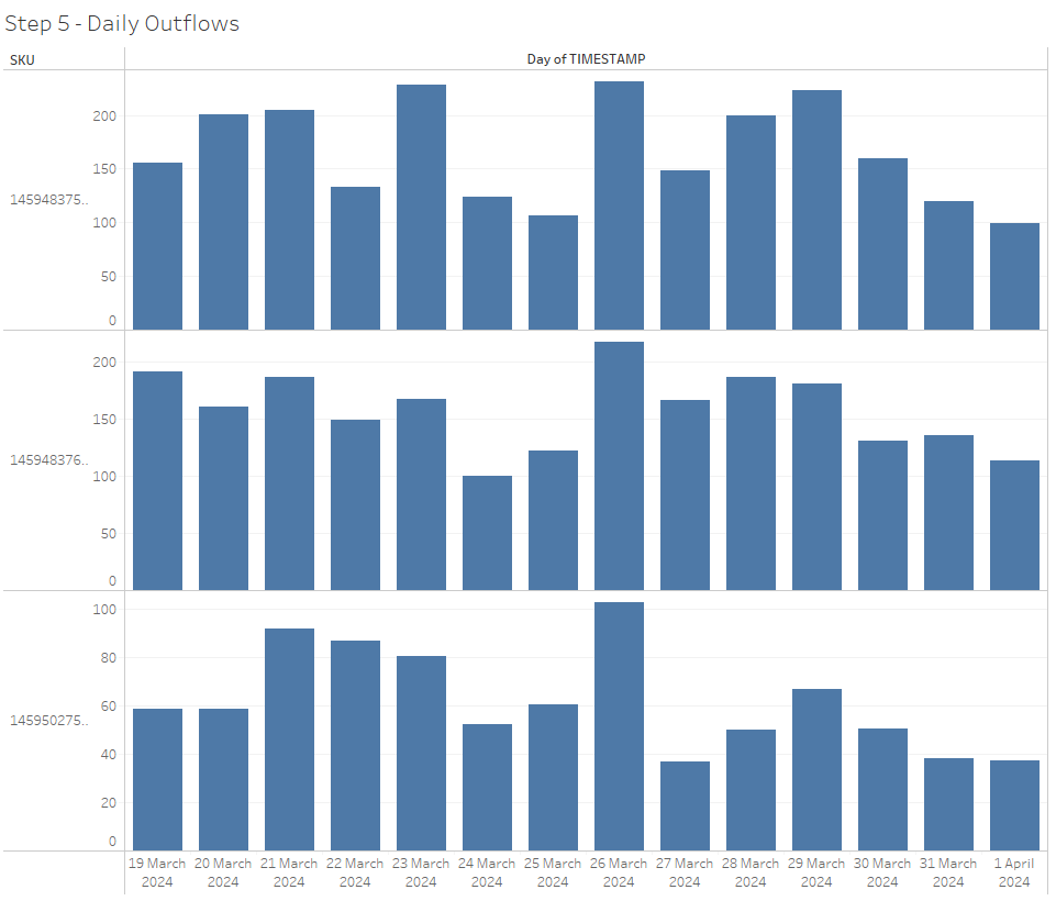
With the interpolated daily values established, we can now use a window function to calculate rolling daily differences, which gives us estimated daily stock outflows for each SKU (potentially indicative of sales).

daily_outflow AS (
    SELECT
        sku,
        timestamp,
        inventory_level, 
        -1 * (inventory_level - 
            LAG(inventory_level, 1, NULL) OVER (PARTITION BY sku ORDER BY timestamp ASC)) AS daily_outflow
    FROM
        interpolation
)

Putting it all together:

WITH calendar_sku_scaffold AS (
  SELECT 
    DATEADD(day, SEQ4(), start_date) AS date
  FROM 
    TABLE(GENERATOR(ROWCOUNT => 10000)), -- Assume a large enough value
    (SELECT 
        DATE_TRUNC('day', MIN(timestamp)) AS start_date,
        DATE_TRUNC('day', MAX(timestamp)) AS end_date
     FROM 
        SCRAPED.PUBLIC.BRAND_A) AS date_range
  WHERE 
    DATEADD(day, SEQ4(), start_date) BETWEEN start_date AND end_date
),

preceding AS (
  SELECT raw_inventories.*,
    scaffold.date
  FROM scaffold
  ASOF JOIN raw_inventories
  MATCH_CONDITION(scaffold.date >= raw_inventories.timestamp)
    ON raw_inventories.product_sku=scaffold.product_sku
),

succeeding AS (
  SELECT raw_inventories.*,
      scaffold.date
  FROM scaffold
  ASOF JOIN raw_inventories
  MATCH_CONDITION(scaffold.date <= raw_inventories.timestamp)
    ON raw_inventories.product_sku=scaffold.product_sku
),

interpolation AS (
    SELECT
      preceding.sku,
      preceding.date AS timestamp,
      preceding.inventory_level 
        + (succeeding.inventory_level - preceding.inventory_level)::FLOAT 
        * (timestampdiff('s', preceding.date, preceding.timestamp)::FLOAT 
           / timestampdiff('s', succeeding.timestamp, preceding.timestamp)::float) AS inventory_level
    FROM preceding
    INNER JOIN succeeding
    WHERE
      preceding.sku = succeeding.sku
      AND preceding.date = succeeding.date
),

daily_outflow AS (
    SELECT
        sku,
        timestamp,
        inventory_level, 
        -1 * (inventory_level - 
            LAG(inventory_level, 1, NULL) OVER (PARTITION BY sku ORDER BY timestamp ASC)) AS daily_outflow
    FROM
        interpolation
)

SELECT
  *
FROM
  daily_outflows

This process transforms the original, messily collected, irregular inventory level data into clean, daily stock outflows:

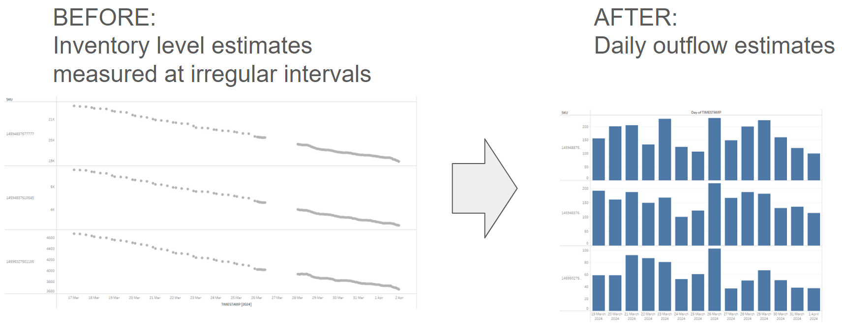
While this article specifically discusses tracking daily inventory outflows, I believe that the transformation pattern described here is broadly applicable to many other scenarios where measurements are taken at irregular intervals using some form of sensor, and there is a need to convert these measurements into estimates with a predefined frequency — think about tracking daily temperature changes for example.

I also must acknowledge that for many problems, this solution may be overengineered and could be considered overkill. Unless we need highly precise estimates for each time interval (hourly, daily, etc.), we can adopt a simpler approach. For instance, we can calculate the mean for each time interval and then take the differences. If the end goal is to estimate quarterly values, then minor hourly discrepancies are unlikely to have a material impact. Ultimately, the complexity of the approach should be justified by the requirements of the goal, otherwise simpler solutions tend to work better.

---

Historically, ASOF joins have been commonly used in purpose-built timeseries databases. More recently mainstream data warehouse platforms started adding support for it as well. As of now, ASOF joins are directly supported by platforms such as DuckDB and Snowflake. BigQuery also supports 'as of' joins, but with a more complex syntax.

For further details on implementation:

• BigQuery

  https://cloud.google.com/bigquery/docs/working-with-time-series#as_of_join

• DuckDB
  https://duckdb.org/docs/guides/sql_features/asof_join.html

• Snowflake

  https://docs.snowflake.com/en/sql-reference/constructs/asof-join